```
// Modified by Edward Brandler, based on original files from PyPortfolioOpt and USolver
```

# <img src=".github/mcportfolio_logo_small.jpg" width="70" height="70" alt="McPortfolio" style="vertical-align: middle;"> McPortfolio - LLM-Driven Portfolio Optimization

This project allows users to work with advanced portfolio optimization using natural language, without writing code. It provides **9 specialized MCP tools** covering everything from classic mean-variance optimization to modern machine learning approaches like Hierarchical Risk Parity.

**Overview of Portfolio Optimizers:**

Portfolio optimizers are algorithms and mathematical tools designed to help investors allocate their capital among different assets in a way that balances risk and return. The most common approaches include:

- **Mean-Variance Optimization (Markowitz):** Finds the portfolio with the lowest risk for a given expected return, or the highest return for a given risk, based on historical means and covariances.
- **Maximum Sharpe Ratio:** Seeks the portfolio with the best risk-adjusted return, maximizing the Sharpe ratio.
- **Minimum Volatility:** Focuses on constructing the portfolio with the lowest possible volatility.
- **Efficient Frontier:** The set of optimal portfolios that offer the highest expected return for a defined level of risk.
- **Black-Litterman Model:** Combines market equilibrium with investor views to produce more stable and realistic portfolios.
- **Hierarchical Risk Parity (HRP):** Uses clustering algorithms to build diversified portfolios that are robust to estimation errors.
- **Mean-CVaR and Mean-Semivariance:** Alternative risk measures that focus on downside risk or tail risk, rather than standard deviation.

These optimizers allow users to tailor their portfolios to their specific risk tolerance, investment goals, and market views.

It gives a universal solver interface for Model-Constraint-Problem (MCP). It makes the [PyPortfolioOpt](https://pyportfolioopt.readthedocs.io/en/latest/) library's features available to Large Language Models (LLMs) through an MCP Server. The main goal is to let .

This project builds on the open-source [USolver](https://github.com/sdiehl/usolver) project, which gives a Model Context Protocol server with tools for different optimization problems. Through USolver, this project works with this powerful solver:

*   [`cvxpy`](https://www.cvxpy.org/) - Used for convex optimization problems in portfolio theory, like maximizing Sharpe ratio or minimizing volatility with linear and quadratic constraints.

## Important Points for LLM-Driven Optimization

The LLM's ability to pick the right solver, parameters, and variables for an optimization problem is a judgment call. It is affected by the non-deterministic nature of LLMs.

**Users should check both the LLM's assumptions and the output.**

### How to Check:
*   **Review the LLM's prompt and generated code/parameters**: Before running, look at the input the LLM is making for the MCP server.
*   **Check server logs**: The MCP server gives detailed logs of operations and parameters used. Review these logs to make sure they match your goals.
*   **Compare with PyPortfolioOpt documentation**: If you know PyPortfolioOpt, check the LLM's chosen parameters and objectives against the library's official docs.
*   **Look at the output metrics**: Check the expected annual return, annual volatility, Sharpe ratio, and other performance metrics to make sure they make sense for your problem.

## Claude Project Instructions

Best practise is to run McPortfolio in a Claude Project. This allows you to set project knowledge, which will improve performance.

There's presently (2025-06-09) no way to force Claude to use a specific tool via MCP Server. So to nudge Claude in the right direction, you can explicitly tell it which tool to use. But even then, you may face issues.

So to help Claude better understand the tools' purposes and how to use them, copy and paste the contents of docs/Claude_Project_Instructions.md to your Claude project's knowledge section. Queries then run from within the project will run more smoothly.

The instructions help Claude to:
- Find when a request fits McPortfolio's features
- Make proper requests using the standard JSON format
- Check outputs against financial best practices
- Give clear explanations of its optimization choices

## An overview of classical portfolio optimization methods

*Reproduced and adapted from [PyPortfolioOpt by robertmartin8](https://github.com/robertmartin8/PyPortfolioOpt?tab=readme-ov-file#an-overview-of-classical-portfolio-optimization-methods)*

Harry Markowitz's 1952 paper is the undeniable classic, which turned portfolio optimization from an art into a science. The key insight is that by combining assets with different expected returns and volatilities, one can decide on a mathematically optimal allocation which minimises the risk for a target return – the set of all such optimal portfolios is referred to as the efficient frontier.

![Efficient Frontier](https://github.com/robertmartin8/PyPortfolioOpt/blob/master/media/efficient_frontier_white.png?raw=true)

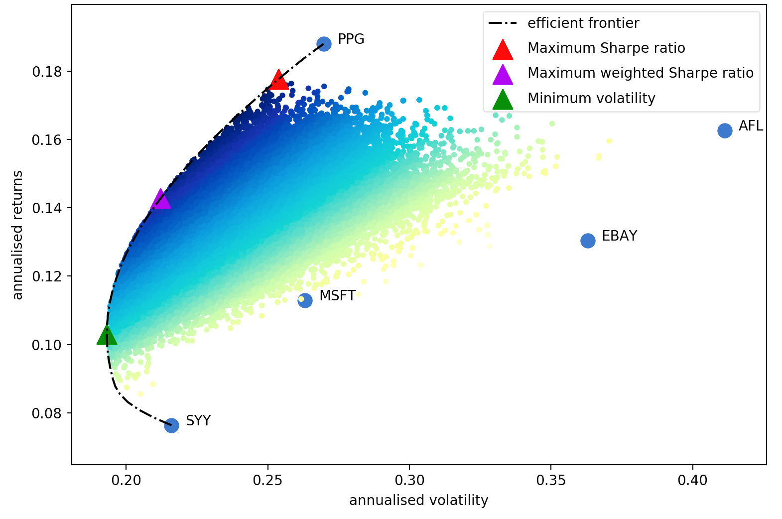
Although much development has been made in the subject, more than half a century later, Markowitz's core ideas are still fundamentally important and see daily use in many portfolio management firms. The main drawback of mean-variance optimization is that the theoretical treatment requires knowledge of the expected returns and the future risk-characteristics (covariance) of the assets. Obviously, if we knew the expected returns of a stock life would be much easier, but the whole game is that stock returns are notoriously hard to forecast. As a substitute, we can derive estimates of the expected return and covariance based on historical data – though we do lose the theoretical guarantees provided by Markowitz, the closer our estimates are to the real values, the better our portfolio will be.

Thus this project provides four major sets of functionality (though of course they are intimately related):

- Estimates of expected returns
- Estimates of risk (i.e covariance of asset returns)
- Objective functions to be optimized
- Optimizers

A key design goal of PyPortfolioOpt is modularity – the user should be able to swap in their components while still making use of the framework that PyPortfolioOpt provides.

## Available MCP Tools

McPortfolio provides a comprehensive suite of portfolio optimization tools through the Model Context Protocol (MCP) server. Each tool is designed for specific optimization scenarios and can be used independently or in combination.

### Core Tools

#### 1. `retrieve_stock_data`
Retrieves historical stock market data for analysis.

**Parameters:**
- `tickers`: List of stock symbols (e.g., ["AAPL", "MSFT", "GOOGL"])
- `period`: Time period for data (e.g., "1y", "2y", "5y")

**Use Case:** Data collection for any portfolio optimization analysis.

#### 2. `solve_portfolio`
General-purpose portfolio optimization with flexible constraints and objectives.

**Parameters:**
- `description`: Problem description
- `tickers`: List of stock symbols
- `constraints`: List of constraint strings (e.g., ["max_weight 0.3", "min_weight 0.05"])
- `objective`: Optimization objective ("minimize_volatility", "maximize_sharpe_ratio", etc.)

**Use Case:** Most common portfolio optimization scenarios with custom constraints.

### Specialized Optimization Methods

#### 3. `solve_efficient_frontier`
Classic Markowitz mean-variance optimization for maximum Sharpe ratio portfolios.

**Parameters:**
- `description`: Problem description
- `tickers`: List of stock symbols
- `min_weight`: Minimum weight per asset (default: 0.0)
- `max_weight`: Maximum weight per asset (default: 1.0)
- `risk_free_rate`: Risk-free rate for Sharpe calculation (default: 0.0)

**Use Case:** Traditional mean-variance optimization, ideal for well-diversified portfolios.

#### 4. `solve_cla`
Critical Line Algorithm for efficient frontier computation.

**Parameters:**
- `description`: Problem description
- `tickers`: List of stock symbols
- `min_weight`: Minimum weight per asset (default: 0.0)
- `max_weight`: Maximum weight per asset (default: 1.0)
- `risk_free_rate`: Risk-free rate for Sharpe calculation (default: 0.0)

**Use Case:** Efficient computation of the entire efficient frontier, useful for risk-return analysis.

#### 5. `solve_hierarchical_portfolio`
Hierarchical Risk Parity (HRP) optimization using machine learning clustering.

**Parameters:**
- `description`: Problem description
- `tickers`: List of stock symbols
- `min_weight`: Minimum weight per asset (default: 0.0)
- `max_weight`: Maximum weight per asset (default: 1.0)
- `risk_free_rate`: Risk-free rate for Sharpe calculation (default: 0.0)

**Use Case:** Modern portfolio construction that addresses estimation errors in traditional optimization.

#### 6. `solve_black_litterman`
Black-Litterman model combining market equilibrium with investor views.

**Parameters:**
- `description`: Problem description
- `tickers`: List of stock symbols
- `views`: List of investor views with expected returns and confidence levels
- `risk_aversion`: Risk aversion parameter (default: 1.0)
- `tau`: Scaling factor for uncertainty (default: 0.05)

**Use Case:** Incorporating market views and expert opinions into portfolio optimization.

### Utility Tools

#### 7. `solve_discrete_allocation`
Converts portfolio weights to actual share quantities for implementation.

**Parameters:**
- `description`: Problem description
- `tickers`: List of stock symbols
- `weights`: Dictionary of target weights (e.g., {"AAPL": 0.4, "MSFT": 0.6})
- `portfolio_value`: Total portfolio value in dollars

**Use Case:** Converting theoretical weights to practical share allocations for trading.

#### 8. `solve_cvxpy_problem`
Advanced custom optimization using CVXPY for complex constraints.

**Parameters:**
- `problem`: CVXPY problem specification with variables, constraints, and objectives

**Use Case:** Custom optimization problems that require advanced mathematical formulations.

#### 9. `simple_cvxpy_solver`
Simplified CVXPY interface for basic optimization problems.

**Parameters:**
- `variables`: List of optimization variables
- `objective_type`: "minimize" or "maximize"
- `objective_expr`: Objective function expression
- `constraints`: List of constraint expressions
- `description`: Problem description

**Use Case:** Simple custom optimization without complex CVXPY knowledge.

## Tool Selection Guide

Choose the right tool based on your optimization needs:

| **Scenario** | **Recommended Tool** | **Why** |
|--------------|---------------------|---------|
| **General portfolio optimization** | `solve_portfolio` | Most flexible, supports various constraints and objectives |
| **Classic mean-variance optimization** | `solve_efficient_frontier` | Standard Markowitz approach, well-tested |
| **Risk parity / diversification focus** | `solve_hierarchical_portfolio` | Modern approach, robust to estimation errors |
| **Efficient frontier analysis** | `solve_cla` | Efficient computation of entire frontier |
| **Incorporating market views** | `solve_black_litterman` | Combines equilibrium with expert opinions |
| **Converting weights to shares** | `solve_discrete_allocation` | Practical implementation of theoretical weights |
| **Custom mathematical constraints** | `solve_cvxpy_problem` | Maximum flexibility for complex problems |
| **Simple custom optimization** | `simple_cvxpy_solver` | Easy interface for basic custom problems |

### When to Use Each Method

**Traditional Approaches:**
- **Efficient Frontier**: When you want to understand risk-return tradeoffs
- **CLA**: When you need the complete efficient frontier efficiently
- **General Portfolio**: When you have specific constraints or objectives

**Modern Approaches:**
- **HRP**: When you have many assets and want robust diversification
- **Black-Litterman**: When you have market views or want to incorporate expert opinions

**Practical Implementation:**
- **Discrete Allocation**: Always use after optimization to convert to actual shares

## Portfolio Optimization Examples

The server provides two main endpoints for portfolio optimization. Here are comprehensive examples for different scenarios:

### 1. Basic Portfolio Optimization

```python
# Example 1: Simple minimum volatility portfolio
{
    "description": "Build a minimum volatility portfolio",
    "tickers": ["AAPL", "MSFT", "NVDA", "GOOGL", "META"],
    "constraints": ["max_weight 0.3"],  # No single stock exceeds 30%
    "objective": "minimize_volatility"
}

# Example 2: Maximum Sharpe ratio portfolio
{
    "description": "Build a maximum Sharpe ratio portfolio",
    "tickers": ["AAPL", "MSFT", "NVDA", "GOOGL", "META"],
    "constraints": ["max_weight 0.3"],
    "objective": "maximize_sharpe_ratio"
}
```

### 2. Sector-Constrained Portfolio

```python
# Example: Diversified portfolio across major sectors
{
    "description": "Build a diversified portfolio across major sectors",
    "tickers": [
        # Technology
        "AAPL", "MSFT", "NVDA", "GOOGL", "META",
        # Financials
        "JPM", "V", "BAC", "GS", "AXP",
        # Healthcare
        "JNJ", "UNH", "PFE", "MRK", "ABBV",
        # Consumer
        "MCD", "PG", "KO", "WMT", "SBUX",
        # Energy
        "XOM", "CVX"
    ],
    "constraints": [
        "max_weight 0.15",     # No single stock exceeds 15%
        "sector_tech 0.35",    # Technology sector max 35%
        "sector_fin 0.35",     # Financial sector max 35%
        "sector_health 0.35",  # Healthcare sector max 35%
        "sector_cons 0.35",    # Consumer sector max 35%
        "sector_energy 0.35"   # Energy sector max 35%
    ],
    "objective": "minimize_volatility"
}
```

### 3. Risk-Constrained Portfolio

```python
# Example: Portfolio with risk constraints
{
    "description": "Build a portfolio with risk constraints",
    "tickers": ["AAPL", "MSFT", "NVDA", "GOOGL", "META", "JPM", "V", "JNJ", "UNH"],
    "constraints": [
        "max_weight 0.2",      # No single stock exceeds 20%
        "min_weight 0.05",     # Each stock must have at least 5%
        "max_volatility 0.15"  # Maximum portfolio volatility of 15%
    ],
    "objective": "maximize_sharpe_ratio"
}
```

### 4. Factor-Constrained Portfolio

```python
# Example: Portfolio with factor constraints
{
    "description": "Build a portfolio with factor constraints",
    "tickers": ["AAPL", "MSFT", "NVDA", "GOOGL", "META", "JPM", "V", "JNJ", "UNH"],
    "constraints": [
        "max_weight 0.2",           # No single stock exceeds 20%
        "min_weight 0.05",          # Each stock must have at least 5%
        "max_beta 1.2",             # Maximum portfolio beta of 1.2
        "min_momentum 0.1",         # Minimum momentum factor exposure
        "max_value 0.3"             # Maximum value factor exposure
    ],
    "objective": "maximize_sharpe_ratio"
}
```

### 5. Custom Risk Measures

```python
# Example: Portfolio with custom risk measures
{
    "description": "Build a portfolio with custom risk measures",
    "tickers": ["AAPL", "MSFT", "NVDA", "GOOGL", "META", "JPM", "V", "JNJ", "UNH"],
    "constraints": [
        "max_weight 0.2",           # No single stock exceeds 20%
        "max_cvar 0.1",             # Maximum Conditional Value at Risk of 10%
        "max_cdar 0.15",            # Maximum Conditional Drawdown at Risk of 15%
        "max_semivariance 0.12"     # Maximum semivariance of 12%
    ],
    "objective": "minimize_volatility"
}
```

### 6. Hierarchical Risk Parity (HRP) Portfolio

```python
# Example: HRP portfolio for risk parity
{
    "description": "Build HRP portfolio for risk parity across sectors",
    "tickers": [
        "AAPL", "MSFT", "GOOGL",  # Tech
        "JPM", "V", "BAC",        # Finance
        "JNJ", "UNH", "PFE",      # Healthcare
        "PG", "KO", "WMT"         # Consumer
    ],
    "min_weight": 0.02,
    "max_weight": 0.25,
    "risk_free_rate": 0.02
}
```

### 7. Critical Line Algorithm (CLA) Portfolio

```python
# Example: CLA optimization for efficient frontier analysis
{
    "description": "Optimize tech portfolio using CLA",
    "tickers": ["AAPL", "MSFT", "GOOGL", "NVDA", "META"],
    "min_weight": 0.05,
    "max_weight": 0.4,
    "risk_free_rate": 0.025
}
```

### 8. Discrete Allocation Example

```python
# Example: Convert weights to actual shares
{
    "description": "Allocate $50,000 based on optimized weights",
    "tickers": ["AAPL", "MSFT", "GOOGL", "NVDA"],
    "weights": {
        "AAPL": 0.35,
        "MSFT": 0.30,
        "GOOGL": 0.20,
        "NVDA": 0.15
    },
    "portfolio_value": 50000
}
```

### 9. Black-Litterman with Market Views

```python
# Example: Black-Litterman with investor views
{
    "description": "Portfolio with bullish view on tech, bearish on energy",
    "tickers": ["AAPL", "MSFT", "GOOGL", "XOM", "CVX", "JPM", "V"],
    "views": [
        {
            "assets": ["AAPL", "MSFT", "GOOGL"],
            "expected_return": 0.15,
            "confidence": 0.8,
            "description": "Tech sector outperformance"
        },
        {
            "assets": ["XOM", "CVX"],
            "expected_return": 0.05,
            "confidence": 0.6,
            "description": "Energy sector underperformance"
        }
    ],
    "risk_aversion": 2.5,
    "tau": 0.025
}
```

### 10. Modern Portfolio Theory (USolver Example)

This project uses USolver for different optimization problems. Here's how it works for a Modern Portfolio Theory problem, turned by the language model into a convex optimization problem that `cvxpy` can solve:

```markdown
Goal: Get the highest expected portfolio return
Rules:

Bonds cannot be more than 40%
Stocks cannot be more than 60%
Real Estate cannot be more than 30%
Commodities cannot be more than 20%
All amounts must be zero or positive
Total must be exactly 100%
Total weighted portfolio risk cannot be more than 10%

Given Data:

Expected returns: Bonds 8%, Stocks 12%, Real Estate 10%, Commodities 15%
Risk factors: Bonds 2%, Stocks 15%, Real Estate 8%, Commodities 20%
```

The language model turns this into a convex optimization problem for `cvxpy`.

$$
\begin{align}
\text{maximize} \quad & 0.08x_1 + 0.12x_2 + 0.10x_3 + 0.15x_4 \\
\text{subject to} \quad & x_1 + x_2 + x_3 + x_4 = 1 \\
& x_1 \leq 0.4 \\
& x_2 \leq 0.6 \\
& x_3 \leq 0.3 \\
& x_4 \leq 0.2 \\
& 0.02x_1 + 0.15x_2 + 0.08x_3 + 0.20x_4 \leq 0.10 \\
& x_1, x_2, x_3, x_4 \geq 0
\end{align}
$$

Where:
- $x_1$ = Bonds amount
- $x_2$ = Stocks amount
- $x_3$ = Real Estate amount
- $x_4$ = Commodities amount

The answer is:

```markdown
Bonds: 30.0%
Stocks: 20.0%
Real Estate: 30.0% (at maximum allowed)
Commodities: 20.0% (at maximum allowed)
Maximum Expected Return: 10.8% annually
```

## Installation

You can install the project using:

```bash
uv run install.py
```

This will install all dependencies and development tools.

To uninstall the project:

```bash
uv run uninstall.py
```

This will remove the project and clean up build artifacts.

### Prerequisites

- Python 3.12 or higher
- [uv](https://github.com/astral-sh/uv) package manager
- Git

### Development Setup

1. Clone the repository:
   ```bash
   git clone https://github.com/ebrandler/mcportfolio
   cd mcportfolio
   ```

2. Create and activate a virtual environment:
   ```bash
   python -m venv .venv
   source .venv/bin/activate  # On Windows: .venv\Scripts\activate
   ```

3. Install development dependencies:
   ```bash
   uv pip install -e ".[dev]"
   ```

4. Install pre-commit hooks:
   ```bash
   pre-commit install
   ```

### Running the Server

**For Claude Desktop/MCP clients (stdio transport):**
```bash
uv run mcportfolio/server/main.py
```

**For HTTP/web deployment:**
```bash
uvicorn mcportfolio.server.main:asgi_app --host 0.0.0.0 --port 8001
```

The HTTP server will be available at `http://localhost:8001`

Test the HTTP server health:
```bash
curl http://localhost:8001/health
```

## Docker Usage

### Building the Image

1. Build the Docker image:
   ```bash
   docker build -t mcportfolio:latest .
   ```

2. Run the container:
   ```bash
   docker run -d -p 8001:8001 --name mcportfolio mcportfolio:latest
   ```

3. Check container status:
   ```bash
   docker ps
   docker logs mcportfolio
   ```

4. Test the HTTP server:
   ```bash
   curl http://localhost:8001/health
   ```

### Docker Compose (Optional)

For development with Docker Compose:

1. Start the services:
   ```bash
   cd infra
   docker-compose up -d
   ```

2. View logs:
   ```bash
   docker-compose logs -f
   ```

3. Stop services:
   ```bash
   docker-compose down
   ```

### Health Checks

The container includes a health check that runs every 30 seconds. You can monitor the health status:

```bash
docker inspect --format='{{.State.Health.Status}}' mcportfolio
```

## Development

### Code Quality

The project uses several tools to maintain code quality:

- `black` for code formatting
- `ruff` for linting
- `mypy` for type checking
- `pytest` for testing
- `pre-commit` hooks for automated checks

Run all checks:
```bash
pre-commit run --all-files
```

### Testing

Run tests with coverage:
```bash
pytest --cov=mcportfolio
```

Generate coverage report:
```bash
pytest --cov=mcportfolio --cov-report=html
```

## Quick Reference

### Available MCP Tools Summary

| Tool | Purpose | Key Parameters |
|------|---------|----------------|
| `retrieve_stock_data` | Get market data | `tickers`, `period` |
| `solve_portfolio` | General optimization | `tickers`, `constraints`, `objective` |
| `solve_efficient_frontier` | Markowitz optimization | `tickers`, `min_weight`, `max_weight` |
| `solve_cla` | Critical Line Algorithm | `tickers`, `min_weight`, `max_weight` |
| `solve_hierarchical_portfolio` | HRP optimization | `tickers`, `min_weight`, `max_weight` |
| `solve_black_litterman` | BL with views | `tickers`, `views`, `risk_aversion` |
| `solve_discrete_allocation` | Weights to shares | `tickers`, `weights`, `portfolio_value` |
| `solve_cvxpy_problem` | Custom optimization | `problem` (CVXPY format) |
| `simple_cvxpy_solver` | Simple custom | `variables`, `objective_expr`, `constraints` |

### Common Objectives
- `minimize_volatility` - Lowest risk portfolio
- `maximize_sharpe_ratio` - Best risk-adjusted returns
- `maximize_return` - Highest expected returns
- `minimize_cvar` - Minimize tail risk

### Common Constraints
- `max_weight 0.3` - No asset exceeds 30%
- `min_weight 0.05` - Each asset at least 5%
- `max_volatility 0.15` - Portfolio volatility ≤ 15%
- `sector_tech 0.4` - Tech sector ≤ 40%

For detailed examples and advanced usage, see the [Portfolio Optimization Examples](#portfolio-optimization-examples) section above.