
Click on "Install Server".
Wait a few minutes for the server to deploy. Once ready, it will show a "Started" state.
In the chat, type
@followed by the MCP server name and your instructions, e.g., "@Optimization MCPallocate a $100k budget across 4 marketing channels to maximize ROI"
That's it! The server will respond to your query, and you can continue using it as needed.
Here is a step-by-step guide with screenshots.
Optimization MCP
Advanced optimization tools for Claude Code - 9 specialized solvers for production use

Version: 2.5.0 (All 4 Enhancements Complete) Status: Production Ready (9 Tools + 1 Orchestration Skill)
Quick Start (60 Seconds)
Want to try it immediately? Here's the fastest path:
1. Install Dependencies (10 seconds)
2. Test It Works (10 seconds)
Run: python test_basic.py
Expected output:
3. Use in Claude Code (30 seconds)
Add to ~/.claude.json:
Restart Claude Code, then try:
4. Next Steps (10 seconds)
Read full documentation below
Explore all 9 tools
Overview
The Optimization MCP provides constraint-based optimization capabilities that integrate seamlessly with your existing Monte Carlo MCP. Find optimal resource allocations, robust solutions across scenarios, and make data-driven decisions under uncertainty.
Key Features
Deep MC Integration: Every tool has native Monte Carlo awareness - use percentile values, expected outcomes, or full scenario distributions
Production Solvers: PuLP (LP/MILP), SciPy (nonlinear), CVXPY (quadratic), NetworkX (network flow)
High Performance: NetworkX provides 10-100x speedup for logistics/routing problems (1K-10K variables)
Zero-Friction Workflows: Optimization outputs feed directly into Monte Carlo validation tools
Open Source: No commercial licenses required (Gurobi/CPLEX not needed)
Production Ready: Internally tested, comprehensive error handling, helpful diagnostics
Comprehensive Coverage: Network flow, Pareto frontiers, stochastic programming, column generation
Pareto Frontier Visualization
Multi-objective optimization balancing conflicting goals (profit vs sustainability):
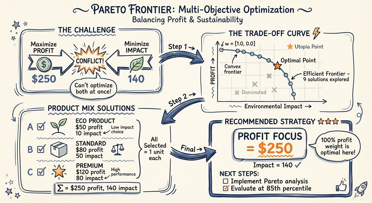
This visualization demonstrates how the Pareto frontier tool explores trade-offs between competing objectives, helping you make strategic decisions across multiple optimal solutions.
Installation
Via Plugin Marketplace (Recommended)
Manual Installation
Auto-Setup: The setup.sh script automatically creates a virtual environment and installs all dependencies.
Important Disclaimers
Software Warranty
This software is provided "as is" under the MIT License, without warranty of any kind, express or implied. The authors are not liable for any damages arising from the use of this software. Always validate optimization results before implementation.
Business Decision Notice
Optimization results are mathematical models based on input data and assumptions. While algorithms are rigorously tested, real-world decisions require:
Validation of results with domain experts
Sensitivity analysis for critical parameters
Testing with historical data before deployment
Understanding of model limitations and assumptions
Financial Advice Disclaimer
The portfolio optimization tool is for educational and analytical purposes only. It does not constitute financial, investment, or professional advice. Consult qualified financial advisors before making investment decisions. Past performance and model outputs do not guarantee future results.
Accuracy and Validation
All optimization tools undergo comprehensive internal testing and validation, but users should:
Verify results independently for critical applications
Test with known problems before production use
Validate assumptions and input data quality
Review solver status and warnings carefully
Consider multiple scenarios and sensitivity analysis
Recommendation: Start with non-critical applications, validate thoroughly, then scale to production use.
Tools
1. optimize_allocation
Purpose: Resource allocation under constraints (budget, time, capacity)
Use Cases:
Marketing budget across channels
Production capacity across products
Project selection with resource limits
Ingredient formulation for beverages/foods
Example:
Monte Carlo Integration:
Parameters:
objective: Dict withitems(list) andsense("maximize"/"minimize")resources: Dict of resource limits (e.g.,{"budget": {"total": 100000}})item_requirements: List of dicts with resource requirements per itemconstraints: Optional additional constraintsmonte_carlo_integration: Optional MC integration (3 modes: percentile, expected, scenarios)solver_options: Optional (time_limit,verbose)
Returns:
status: "optimal", "infeasible", "unbounded", or "error"objective_value: Optimal valueallocation: Dict of selected items (1 = selected, 0 = not)resource_usage: Utilization stats for each resourceshadow_prices: Marginal value of relaxing each constraintmonte_carlo_compatible: Output formatted for MC validation
Multi-Objective Optimization
NEW in v1.1.0: Optimize for multiple competing objectives with weighted scalarization.
Use Cases:
Balance profit and sustainability
Trade off return vs. risk
Optimize cost and quality simultaneously
Any multi-criteria decision problem
Example:
Requirements:
At least 2 objective functions required
Weights must sum to 1.0 (within 0.01 tolerance)
Each weight must be between 0 and 1
Each function has its own
itemslist withnameandvalue
Backward Compatible: Single-objective format still works exactly as before.
Enhanced Constraints
NEW in v2.0.0: Advanced constraint types for complex decision logic.
Constraint Types:
1. Conditional (If-Then):
2. Disjunctive (OR - At Least N):
3. Mutual Exclusivity (Exactly N):
Combined Example:
Use Cases:
Product bundling rules
Technology dependency chains
Strategic option selection
Regulatory compliance constraints
2. optimize_robust
Purpose: Find robust solutions that work well across Monte Carlo scenarios
Use Cases:
Allocation that works in 85%+ of scenarios
Worst-case optimization
Risk-constrained decisions
Example:
Parameters:
objective,resources,item_requirements: Same as optimize_allocationmonte_carlo_scenarios: Dict withscenarioslist from MC outputrobustness_criterion: "best_average", "worst_case", or "percentile"risk_tolerance: Float (0-1), e.g., 0.85 = works in 85% of scenariosconstraints,solver_options: Optional
Returns:
allocation: Robust allocation decisionrobustness_metrics: Performance statistics across scenariosoutcome_distribution: List of outcomes for validationmonte_carlo_compatible: Output for MC tools
3. optimize_portfolio
NEW in v2.0.0: Portfolio optimization with risk-return tradeoffs using quadratic programming.
Purpose: Optimize investment portfolio allocation considering correlations and risk
Use Cases:
Investment portfolio allocation
Asset selection with risk-return tradeoffs
Sharpe ratio maximization
Efficient frontier construction
Optimization Objectives:
Sharpe Ratio: Maximize (return - risk_free) / risk
Min Variance: Minimize portfolio risk for target return
Max Return: Maximize return for target risk
Example 1: Sharpe Ratio Optimization:
Example 2: Minimum Variance:
Example 3: Maximum Return:
Parameters:
assets: List of{"name": str, "expected_return": float}covariance_matrix: N×N matrix of asset return covariancesoptimization_objective:"sharpe","min_variance", or"max_return"risk_free_rate: Risk-free rate for Sharpe (default: 0.02)constraints: Optional:max_weight: Max weight per asset (e.g., 0.30 = 30%)min_weight: Min weight per asset (e.g., 0.05 = 5%)target_return: Required formin_varianceobjectivetarget_risk: Required formax_returnobjectivelong_only: Prevent short selling (default: True)
monte_carlo_integration: Optional MC integrationsolver_options: Optional solver settings
Returns:
status: Optimization statusweights: Dict of optimal portfolio weights (sum to 1.0)expected_return: Portfolio expected returnportfolio_variance: Portfolio variance (risk²)portfolio_std: Portfolio standard deviation (risk)sharpe_ratio: (return - rf) / stdassets: Asset-level details with risk contributionsmonte_carlo_compatible: MC validation output
Solver: CVXPY with SCS (handles quadratic objectives and constraints)
4. optimize_schedule
NEW in v2.0.0: Task scheduling with dependencies and resource constraints.
Purpose: Optimize project schedules considering task dependencies, resource limits, and temporal constraints
Use Cases:
Project scheduling (RCPSP)
Job shop scheduling
Task prioritization with deadlines
Resource allocation over time
Optimization Objectives:
Minimize Makespan: Complete project as fast as possible
Maximize Value: Prioritize high-value tasks within time budget
Example 1: Software Project Schedule:
Example 2: With Deadlines:
Parameters:
tasks: List of tasks with:name: Task identifierduration: Time units requiredvalue: Task value/priority (optional, for maximize_value)dependencies: List of prerequisite task names (optional)resources: Resource requirements per time unit (optional)
resources: Available resources per time periodtime_horizon: Total scheduling windowconstraints: Optional temporal constraints:Deadline: Task must finish by time T
Release: Task cannot start before time T
Parallel limit: Max N tasks simultaneously
optimization_objective:"minimize_makespan"or"maximize_value"monte_carlo_integration: Optional MC for uncertain durationssolver_options: Optional solver settings
Returns:
status: Optimization statusschedule: Dict mapping task → start_timemakespan: Project completion time (for minimize_makespan)total_value: Sum of scheduled task values (for maximize_value)resource_usage: Resource utilization timelinecritical_path: Task sequence determining makespantasks: Task-level details with critical path markersmonte_carlo_compatible: MC validation output
Solver: PuLP with CBC (MILP for task-time assignment)
5. optimize_execute
NEW in v2.1.0: Custom optimization with automatic solver selection and flexible problem specification.
Purpose: Power user tool for rapid prototyping and custom optimization problems
Use Cases:
Custom optimization formulations not fitting standard templates
Rapid prototyping of new optimization problems
When you know the mathematical form and want automatic solver selection
Educational/research applications
Key Features:
Auto-Solver Selection: Automatically detects and selects best solver (PuLP/SciPy/CVXPY)
Flexible Specification: Dict-based problem definition
All Solvers Accessible: Can override auto-detection to force specific solver
Example 1: Simple Knapsack Problem:
Example 2: With Solver Override:
Parameters:
problem_definition: Dict with:variables: List of{"name": str, "type": "continuous"|"integer"|"binary", "bounds": (lower, upper)}objective:{"coefficients": {var: coeff}, "sense": "maximize"|"minimize"}constraints: List of{"coefficients": {var: coeff}, "type": "<="|">="|"==", "rhs": number}
auto_detect: Auto-select best solver (default: True)solver_preference: Override with"pulp","scipy", or"cvxpy"monte_carlo_integration: Optional MC integrationsolver_options: Optional (time_limit,verbose)
Returns:
status: Optimization statussolver_used: Which solver was selectedobjective_value: Optimal valuesolution: Dict of variable valuessolve_time_seconds: Solve timeproblem_info: Problem statisticsshadow_pricesordual_values: Sensitivity information (solver-dependent)monte_carlo_compatible: MC validation output
Auto-Detection Logic:
Has binary/integer variables → PuLP (CBC)
Continuous linear → PuLP (default)
Can override with
solver_preferenceparameter
When to Use:
✅ You have a custom problem not fitting standard templates
✅ You want to prototype quickly with dict specification
✅ You need access to all 3 solvers from one interface
✅ You're comfortable with mathematical formulation
When NOT to use:
❌ Standard allocation → Use optimize_allocation instead
❌ Portfolio → Use optimize_portfolio instead
❌ Scheduling → Use optimize_schedule instead
Solver: Auto-selected (PuLP/SciPy/CVXPY) or manual override
Why optimize_execute is Your "Escape Hatch"
The Flexibility Layer: While specialized tools cover 90% of use cases, optimize_execute is deliberately designed for the other 10%.
When specialized tools fit (use these first):
Budget allocation →
optimize_allocationPortfolio →
optimize_portfolioScheduling →
optimize_scheduleNetwork routing →
optimize_network_flowMulti-objective trade-offs →
optimize_pareto
When you need custom formulation (use optimize_execute):
Custom knapsack variants
Unusual constraint types
Rapid prototyping of new problems
Educational/research applications
Any problem not fitting standard templates
Think of it as:
Specialized tools = High-level API (easy, opinionated, 90% of cases)
optimize_execute = Low-level API (flexible, general, 10% of cases)
Example - Custom Multi-Dimensional Knapsack:
You get:
Auto-detection of solver (PuLP for this binary problem)
All the power of mathematical programming
None of the boilerplate of specialized tools
Monte Carlo integration still available
Both have their place - use specialized tools when they fit (easier, better validation), optimize_execute when you need full control.
6. optimize_network_flow
NEW in v2.2.0: Network flow optimization with specialized NetworkX algorithms for 10-100x speedup.
Purpose: Solve network flow problems (min-cost flow, max-flow, assignment)
Use Cases:
Supply chain routing (warehouse → customer distribution)
Transportation logistics (minimize shipping costs)
Assignment problems (workers to tasks, machines to jobs)
Maximum throughput/capacity problems
Key Features:
High Performance: NetworkX specialized algorithms 10-100x faster than general LP
Auto-Solver Selection: NetworkX for pure network flow, PuLP fallback for complex constraints
Bottleneck Analysis: Identifies capacity-constrained edges
Node Balance Tracking: Flow conservation verification at each node
Example 1: Supply Chain Min-Cost Flow:
Example 2: Maximum Flow:
Example 3: Assignment Problem:
When to Use:
✅ Pure network flow problems (routing, logistics, assignment)
✅ Large-scale problems (1K-10K variables) where speed matters
✅ Supply chain optimization with transportation costs
✅ Capacity/throughput maximization
When NOT to use:
❌ Multi-commodity flow (different product types) → Use optimize_allocation
❌ Complex side constraints beyond flow conservation → optimize_execute with PuLP
Solver: NetworkX (primary) with PuLP fallback for complex cases Performance: <0.001s for 100 nodes, <2s for 1000 nodes
7. optimize_pareto
NEW in v2.3.0: Pareto multi-objective optimization - explore full trade-off frontier.
Purpose: Generate complete Pareto frontier showing all trade-offs between conflicting objectives
Use Cases:
Strategic planning (profit vs sustainability vs risk)
Design optimization (cost vs quality vs time)
Product selection (revenue vs customer satisfaction)
Multi-criteria decision support
Key Features:
Full Frontier Generation: 20-100 non-dominated solutions (not just one weighted point)
Knee Point Recommendation: Automatically identifies best balanced solution
Trade-Off Analysis: Quantifies marginal rates of substitution between objectives
Mixed Senses: Handles maximize + minimize objectives simultaneously
Example: Profit vs Sustainability Trade-Off:
When to Use:
✅ Don't know the "right" trade-off weights upfront
✅ Need to show executives/stakeholders multiple options
✅ Want to understand sensitivity to objective priorities
✅ Multi-criteria decision problems
When NOT to use:
❌ Already know exact weights → Use optimize_allocation with multi-objective
❌ Single objective → Use optimize_allocation
Solver: PuLP (solves weighted sums systematically) Performance: ~0.5-2s for 20 frontier points
Scalability Guidelines
Understanding the performance characteristics of each tool helps you choose the right approach and set realistic expectations.
optimize_allocation
Recommended limits:
Items: <500 (optimal performance)
Resources: <100
Binary/integer variables: <1000
Constraints: <1000
Performance characteristics:
Uses PuLP with CBC solver (branch-and-cut MIP)
Small problems (<50 items): <1 second
Medium problems (50-500 items): <10 seconds
Large problems (500-1000 items): <60 seconds
When to use: Budget allocation, resource assignment, selection problems
optimize_robust
Recommended limits:
Items: <100 (candidate generation is combinatorial)
Scenarios: <1000
Total evaluations (items × scenarios): <100,000
Performance characteristics:
Generates candidate allocations, evaluates across scenarios
Evaluation time grows linearly with scenarios
Candidate generation can be exponential in items
When to use: Risk-aware allocation under uncertainty
optimize_portfolio
Recommended limits:
Assets: <500
Covariance matrix: N×N must fit in memory (~500×500 = 2MB)
Performance characteristics:
Uses CVXPY with SCS/OSQP solvers (quadratic programming)
Small portfolios (<50 assets): <1 second
Medium portfolios (50-200 assets): <5 seconds
Large portfolios (200-500 assets): <30 seconds
When to use: Investment portfolio optimization, risk-return trade-offs
optimize_schedule
Recommended limits:
Tasks: <50
Time horizon: <100 periods
Total time-indexed variables (tasks × horizon): <5000
Performance characteristics:
Uses time-indexed formulation (binary variable per task-time pair)
Variables = tasks × time_horizon
Small projects (<20 tasks): <10 seconds
Medium projects (20-50 tasks): <60 seconds
When to use: Project scheduling, resource-constrained planning
optimize_network_flow
Recommended limits:
Nodes: <10,000
Edges: <100,000
Performance characteristics:
Uses NetworkX specialized algorithms (network simplex, Edmonds-Karp)
Exploits network structure for 100-5000x speedup vs general LP
Small networks (<100 nodes): <0.1 seconds
Medium networks (100-1000 nodes): <1 second
Large networks (1000-10000 nodes): <10 seconds
When to use: Transportation, logistics, routing, assignment problems
optimize_pareto
Recommended limits:
Frontier points: 20-100 (more points = finer trade-off curve)
Items: Same as optimize_allocation
Objectives: 2-4 (visualization becomes difficult beyond 3)
Performance characteristics:
Solves one optimization per frontier point
Total time ≈ single optimization × number of points
20 points typically takes 10-30 seconds
When to use: Multi-objective trade-off analysis, exploring decision space
optimize_stochastic
Recommended limits:
Scenarios: <200 (extensive form size scales linearly)
First-stage variables: <500
Second-stage variables: <500
Total problem size: n₁ + S×n₂ < 100,000
Performance characteristics:
Uses 2-stage extensive form (single large LP)
Problem size = first_stage + scenarios × second_stage
50 scenarios, 100 vars/stage: ~5 seconds
200 scenarios, 200 vars/stage: ~60 seconds
When to use: Sequential decisions with uncertainty revelation (inventory, capacity planning)
optimize_column_gen
Recommended limits:
Master problem variables: <10,000 (framework ready, user implements pricing)
Iterations: <100
Performance characteristics:
Framework for large-scale problems (>1000 variables)
Performance depends on user-provided pricing subproblem
Currently returns with initial columns (placeholder pricing)
When to use: Very large problems, cutting stock, crew scheduling (requires custom pricing)
optimize_execute
Recommended limits:
Variables: Depends on auto-detected solver
PuLP (LP/MIP): <10,000 variables
SciPy (nonlinear): <1,000 variables
CVXPY (QP): <5,000 variables
Performance characteristics:
Auto-detects problem type and selects appropriate solver
Performance matches selected backend solver
When to use: Custom problems not covered by specialized tools
Performance Tips
Start small: Test with 10-20% of full problem size first
Use network_flow for network problems: 100-5000x faster than general LP
Reduce scenarios: 50 scenarios often sufficient for stochastic problems
Use robust over stochastic for simple cases: Faster evaluation, no extensive form
Pareto frontier: 20 points usually sufficient to see trade-off curve
Check solver_options: Set
time_limitto prevent runaway solves
When You Hit Scale Limits
If your problem exceeds recommended limits:
Decomposition: Break into smaller subproblems
Aggregation: Group similar items/resources
Sampling: Use subset of scenarios for stochastic
Heuristics: Use optimize_robust with candidate sampling
Column generation: Use optimize_column_gen for very large problems
Commercial solvers: Consider Gurobi/CPLEX for 10x+ speedup (not included)
Monte Carlo Integration Patterns
This MCP has deep Monte Carlo integration - every tool can work with uncertainty. However, tools use different patterns based on their needs.
Pattern Summary
Tool | MC Parameter | Modes Supported | Purpose |
optimize_allocation | monte_carlo_integration | percentile, expected | Use MC values in objective |
optimize_robust | monte_carlo_scenarios | scenarios only | Evaluate across all scenarios |
optimize_portfolio | monte_carlo_integration | percentile, expected | Use MC returns/covariance |
optimize_schedule | monte_carlo_integration | percentile, expected | Use MC durations |
optimize_execute | monte_carlo_integration | percentile, expected | Use MC coefficients |
optimize_network_flow | monte_carlo_integration | percentile, expected | Use MC costs/capacities |
optimize_pareto | monte_carlo_integration | percentile, expected | Use MC objective values |
optimize_stochastic | scenarios | scenarios only | Model uncertainty explicitly |
Pattern Type A: Percentile/Expected (Most Tools)
Used by: allocation, portfolio, schedule, execute, network_flow, pareto
Purpose: Extract specific values (P10/P50/P90 or expected) from MC output and use in optimization
Example:
Modes:
"percentile": Use P10/P50/P90 values from distributionP10 = Conservative (pessimistic)
P50 = Base case (median)
P90 = Optimistic
"expected": Use mean values from distribution
What happens: Tool extracts specified percentile/expected values from mc_output and uses them in optimization
Pattern Type B: Scenarios (Robust & Stochastic)
Used by: optimize_robust, optimize_stochastic
Purpose: Evaluate decisions across ALL scenarios (not just one percentile)
Example for optimize_robust:
Example for optimize_stochastic:
What happens: Tool evaluates optimization across all scenarios
optimize_robust: Tests candidate allocations against all scenariosoptimize_stochastic: Models uncertainty explicitly in 2-stage formulation
When to Use Which Pattern
Use Pattern A (percentile/expected) when:
You want a single deterministic optimization
You're comfortable picking P10/P50/P90 upfront
You want fast solve times
Example: "Allocate budget using median ROI values"
Use Pattern B (scenarios) when:
You want robustness across uncertainty
You care about worst-case or risk tolerance
You need sequential decisions with uncertainty revelation
Example: "Find allocation that works in 85% of scenarios"
Common Workflows
Workflow 1: Conservative Planning
Workflow 2: Robust Optimization
Workflow 3: Stochastic Sequential Decisions
Migration Guide
If you're using the old pattern and want to update:
Old (still works):
New (with MC):
Backward compatible: All tools work without MC parameters (deterministic mode)
Schema Grammar Reference
Common data structures used across multiple tools. Learn once, use everywhere.
Resource Definition
Used in: optimize_allocation, optimize_schedule, optimize_pareto, optimize_stochastic, optimize_robust
Format:
Examples:
Item Requirements
Used in: optimize_allocation, optimize_robust, optimize_pareto
Format:
Examples:
Important: Resource names in requirements must match resource names in resources dict
Objective Specification
Used in: optimize_allocation, optimize_robust, optimize_pareto
Single Objective Format:
Multi-Objective Format (allocation only):
Example:
Constraint Specification
Used in: optimize_allocation, optimize_schedule
Format:
Examples:
Network Specification
Used in: optimize_network_flow
Format:
Example:
Node types:
Source:
supply > 0(produces flow)Sink:
demand > 0(consumes flow)Transshipment: Neither supply nor demand (passes flow through)
Solver Options
Used in: All tools
Format:
Example:
Usage:
Canonical Workflows
Workflow 1: Optimize → Validate → Robustness Test
Find optimal allocation, validate with Monte Carlo, test assumption robustness.
Workflow 2: MC Scenarios → Robust Optimization
Generate scenarios with Monte Carlo, optimize for robustness.
Technical Architecture
Solvers
Solver | Type | Best For | Scale |
PuLP + CBC | LP/MILP | Resource allocation, scheduling, formulation | Up to 10,000 vars |
SciPy | Nonlinear | Continuous optimization with bounds/constraints | 10-1000 vars |
File Structure
Performance Targets
Problem Size | Target Time | Use Case |
Small (< 50 vars) | < 1 sec | Formulation problems |
Medium (50-500 vars) | < 10 sec | Resource allocation |
Large (500-1000 vars) | < 60 sec | Complex scheduling |
Troubleshooting
MCP Not Loading
Check configuration:
grep -A5 '"optimization-mcp"' ~/.claude/config/mcp-profiles.jsonVerify server.py is executable:
ls -l ~/.claude/mcp-servers/optimization-mcp/server.pyCheck logs:
tail -f /tmp/optimization-mcp.log
Infeasible Problems
If you get status: "infeasible":
Check that at least one item fits within resource limits
Verify constraints aren't contradictory
Use smaller problem to debug
Slow Solving
If optimization takes > 60 seconds:
Reduce problem size (fewer items/constraints)
Add
solver_options: {"time_limit": 30}to stop earlyConsider breaking into subproblems
Roadmap
Week 2 (Next Steps)
Tool 3:
optimize_portfolio- Portfolio optimization with Sharpe ratioTool 4:
optimize_schedule- Task scheduling with dependenciesCVXPY integration for quadratic objectives
Week 3
Tool 5:
optimize_execute- Custom workflows with code executionOrchestration skill:
robust-optimization- End-to-end automationPerformance benchmarks and optimization
Examples
Example 1: Marketing Budget Allocation
Dependencies
mcp >= 0.9.0 - Model Context Protocol
pulp >= 2.7.0 - Linear/integer programming
scipy >= 1.16.0 - Scientific computing
numpy >= 2.3.0 - Numerical arrays
pytest >= 7.0.0 - Testing framework
License
Part of Claude Code MCP ecosystem. Use responsibly.
Support
Issues: Report problems in your Claude Code setup
Documentation: See plan file at
~/.claude/plans/resilient-frolicking-wreath.mdExamples: Check
examples/directory for complete workflows
Week 1 Status: ✓ Production Ready with 2 Core Tools
Next: Week 2 - Portfolio optimization and scheduling tools